The Road to the Eu’s +2^oc Maximum Temperature Limit
Andrew Glikson [0]
Earth and paleoclimate scientist
Australian National University

Taking into account the (1) masking effect of industry-emitted sulphur aerosols, and (2) lost reflectance (albedo) due to Arctic Sea ice melt and other parts of the polar and mountain glaciers, global temperature-equivalents are tracking close to the European Union maximum permissible level of 2 degrees Celsius.

________________________________________________________________________________________________

According to the IPCC AR4-2007 report [1] a total anthropogenic greenhouse factor of 3.06 Watt/m2, equivalent to about +2.3 degrees C, is masked by a compensating aerosol albedo effect of -1.25 Watt/m2 (mainly sulphur from industrial emissions) equivalent to about -0.9C (without land clearing albedo gain and ice melt albedo loss) (Table 1). Once the short-lived aerosols dissipate, adding the reflectance loss of melting polar ice (where maximum warming of up to 4 degrees C occurs; Figure 2), mean global temperatures track toward +2 degrees C, considered by the European Union to be the maximum permissible level.

From Table 1, subtracting the aerosol masking effect, the magnitude of the 1750 – 2005 mean forcing at ~3 Watt/m2 is approaching 50% of the total last glaciation termination of 6.5+/-1.5 Watt, not accounting for developments since 2005. This includes the reduction in albedo due to melting of Arctic Sea ice and other parts of the cryosphere.

Since the mid-1990s the mean global temperature trend has become increasingly irregular, representing an increase in climate variability with global warming, as reflected by variations in the ENSO cycle and oscillating ice melt and re-freeze cycles. The solar sunspot cycle effect is at about +/-0.1 degrees C, an order of magnitude less than greenhouse forcing. Sharp peaks include the 1998 El-Nino peak (near +0.55C) and the 2007 La Nina trough (near -0.7C) [2]. Mean global temperature continued to rise during 1999-2005 by about 0.2C (Figure 3).

The effects of this warming on the cryosphere include:

(A) Reduction in the Arctic Sea multi-year ice cover from about 4.2 to 2.5 million square km during 2000-2009 [3] (Figure 4).

(B) Increase in Greenland September ice melt area from 350,000 to 550,000 square km during 1997-2007 [4] (Figure 5).

(C) Warming of the entire Antarctic continent by 0.6C and of west Antarctic by 0.85C during 1957-2006 [5], reflected by collapse of west Antarctic ice shelves [6] (Figure 6).

Variations in temperature and sea ice cover around Antarctica are effected by the shrinking polar wind vortex and tropospheric and stratospheric ozone layer conditions, resulting in geographic and temporal variability in sea and land ice cover (Figure 7).

Ongoing global warming may lead to the release of methane from permafrost, collapse of the North Atlantic Thermohaline current, high-energy weather events and yet little-specified shifts in atmospheric states (tipping points) [7]

 

Table 1. Comparisons between anthropocene (1750-2005), last glacial termination (20 – 11.7 kyr) and Pliocene (~3 Ma) CO2 levels, climate forcings, mean global temperatures and sea levels. Sources: [1] and [19].

 

Period	CO2 ppm	Forcings Watt/m2	Temperature oC (1oC ~ ¾ W/m2)	Sea level metres
1750 – 2005	260-387	Greenhouse: +3.06 Albedo: -1.25* Current balance: +1.81 Ice albedo loss (? W/m2)	~ +2.3 ~ -0.9 ?ToC	Tracking toward Pliocene levels
Last glacial termination (20 – 11.7 kyr	180-280	Greenhouse gases: +3.0+/-0.5 Ice sheets and vegetation albedo loss: +3.5+/-1.0.	~ +5.0+/-1.0	+120
Pliocene (3 Ma)	400		+2 to 3	+25 +/-12

*(not including land clearing)

 

This experiment by Homo “sapiens” is a novel one. Developments may include periods of cooling, as may be indicated by the current slow-down of Greenland glaciers. In a recent paper by Dakos et al. (2008) abrupt climate changes in the past are shown to have been preceded by quiet periods [8].

”Skeptics” use such short-term variability, for example slowing down of Greenland glaciers, to argue “global cooling” and thereby a “justification” for further carbon emissions [9 – 11].

The implications of climate change for ecosystems are illustrated in the new book Heatstroke: Nature in an Age of Global Warming [1] by Anthony Barnosky, of Yale University, who states:

I think probably the biggest cause for worry is we really are seeing the disappearance of whole ecological niches, which means extinctions." [12]

Despite intensified warnings from the Copenhagen climate conference [13], as a self-fulfilling prophecy the government’s “great moral issue of our time” [14] is being relegated to secondary priority [15].

Given that warnings by scientists have proven mostly correct, as contrasted with watered-down reports percolating upward through bureaucracies, there is little evidence the Rudd government is listening to the recent dire warnings by climate scientists [16].

The decline by CSIRO to report directly to the recent Senate climate inquiry [17], reminiscent of the Howard era [18], has only been saved by the courage of individual scientists, one of whom compared Labor's targets to "Russian roulette with the climate system with most of the chambers loaded".

References [1]

 

 

Figure 1.

IPCC 2007 Figure SPM.2. AR4-WG1-2007 - Global average radiative forcing (RF) estimates and ranges in 2005 for anthropogenic carbon dioxide (CO2 ), methane (CH4 ), nitrous oxide (N2O) and other important agents and mechanisms. The net anthropogenic radiative forcing and its range are also shown. Volcanic aerosols contribute an additional natural forcing but are not included in this figure due to their episodic nature.

 

 

Figure 2. NASA-GISS Land-Ocean temperature anomaly showing the strongest temperature anomalies occur over polar winters. (A) End of NH summer: September, 2008 relative to 1951-1980. Mean global anomaly 0.52^oC. Note the high early-summer temperatures over Antarctica. (B) End NH winter: April 2009 relative to 1951-1980 baseline. Mean global anomaly: 0.43^oC. Note the increase in temperatures over +4^oC over eastern Siberia and a decrease by more than over -2^oC over East Antarctica.

 

 

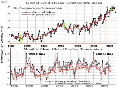
Figure 3. Mean global temperature changes (NASA/GISS).

1880 – 2009 annual mean and 5-year annual mean temperatures 1996 – 2009 monthly meteorological stations and Land-Ocean temperatures. index.

Note the 1998 El-Nino anomaly and 2008 La-Nina anomaly.

 

 

Figure 4 [2]. The decline in multiyear (including second-year ice) sea ice coverage measured by NASA’s QuikScat satellite from 1999 to 2009. Each field shows the coverage on January 1 of that year. There is a 40 percent drop in coverage between 2005 and 2007.

 

 

Figure 5 [3]. Change in the extent of Greenland ice melt areas from 350,000 km² in September 1997 to 550,000 km² in September 2007

 

 

Figure 6 [4]. The Antarctic continent (upper image) and temperature changes per decade during 1958 – 2008 (lower image). Note the contrast between west and east Antarctica and the internal variations of warming and slightly cooling regions in east Antarctica.

 

 

Figure 7 (A) Antarctic sea ice extent [5] during SH Winter (September, 1999) and summer (February, 2009). (B) Sea ice per cent concentration trends around Antarctica for October 2008 relative to 1979-2000 October monthly average. National Snow and Ice Data Centre [6].